Save
•
•Save As
the first time and give your workbook a name. Use the Save
(diskette icon) to save any changes to your worksheet.
•
![]() Save OFTEN!!!
Save OFTEN!!!
Worksheet and Booklets
• When you start a new Excel document, you are opening a blank booklet.
• There are 3 worksheets already available.
•
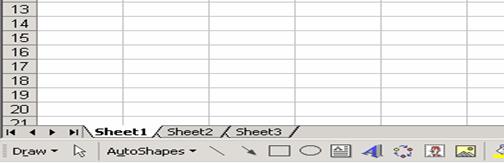 You
can insert more or delete ones you don’t need.
You
can insert more or delete ones you don’t need.

Page Setup


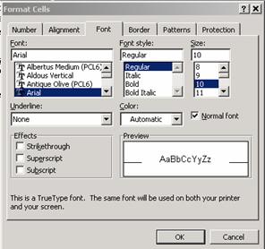
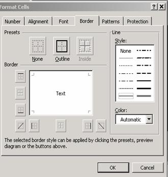
Highlight and Format

Format


Adjusting Rows and Columns

 Fill in

 Auto Fill

![]()
![]()
 Insert
a Picture
Insert
a Picture
 Sort
Sort


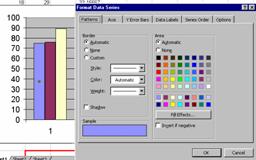
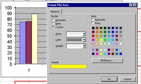
Chart


ü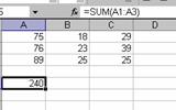
![]()
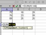
 Formulas
ü